This is the first in a multi-part series on repurposing old EMC equipment.  I recently acquired six  EMC Centera nodes, two of the nodes with 4x1TB SATA drives and four of the nodes with 4x500GB SATA drives so I started thinking what can I do with these Pentium based machines with 1 GB of RAM and a boat load of storage.  An idea hit me to create a NAS share leveraging a global file system to aggregate the capacity and performance across all the Centera nodes.  Seemingly simple there was a challenge here, most modern day global file systems like GlusterFS or GFS2 require a 64 bit processor architecture, the Centera nodes use 32 bit Pentium processors.  After spending a vacation day researching I identified two possible Global file systems as potential options, XtreemFS and FraunhoferFS (fhgfs).  I discovered fhgfs first and it looked pretty interesting, a fairly traditional Global File System consisting of metadata nodes and storage nodes (I came across this presentation which provides a good overview of the FraunhoferFS.  While fhgfs provided the basics of what I was looking for the missing link was how I was going to protect the data, fhgfs for the most part relied on hardware RAID for node survivability, because the Centera nodes are built to run EMC’s CentraStar an OS which leverages RAIN (Redundant Array of Independent Nodes) no redundancy is built in at the node level.  EMC acquired Centera and CentraStar from a Belgian company named FilePool in 2002.  As I thought trough some possible workarounds I stumbled across XtreemFS an interesting object based global file system, what was most interesting was the ability to replicate objects for redundancy.  At this point I decided to attempt to move forward with XtreemFS, my single node install went well, no issues  to really speak of as I moved towards the multi node configuration I was beginning to get core dumps when starting the daemons, is was at this point that I decided to give fhgfs a try, thinking that in phase 2 of the project I could layer on either rsync of drbd to protect the data (not there yet so not sure how well this theory will play out).  The fhgfs installed fairly easily and is up and running, the rest of this blog will walk you though the steps that I took to prepare the old Centera nodes, install Ubuntu and configure Ubuntu server, install an configure fhgfs.

Because the Centera nodes came out of a production environment they were wiped prior to leaving the production data center (as a side note DBAN booted form a USB key was used to perform the wipe of each node).  So with no data on the four Centera node internal drives the first step was to install a base OS on each node.  Rather than use a USB CD-ROM (only had one) I decided to build a unattended PXE boot install.

Phase 1:  Basic Environment Prep:

Step 1:  Build PXE Server (because this is not a blog on how to build a PXE server I suggest doing some reading).  The following two links should be very helpful:  https://help.ubuntu.com/community/PXEInstallServer, https://help.ubuntu.com/community/PXEInstallMultiDistro. I built my PXE boot server on Ubuntu 12.04 server but the process in pretty much as documented in the above two links.  You can also Google “ubuntu pxe boot server”.

Note:  One key is to be sure to install Apache and copy your Ubuntu distro to a http accessible path.  This is important when creating your kickstart configuration file (ks.cfg) so you can perform a completely automated install.  My ks.cfg file.

Step 1A:  Enter BIOS on each Centera and reset to factory defaults, make sure that each node has PXE boot enabled on the NICs.

Note:  I noticed on some of the nodes that the hardware NIC enumeration does not match Ubuntu’s ETH interface enumeration (i.e. – On 500GB nodes ETH0 is NIC2) just pay attention to this as it could cause some issues, if you have the ports just cable all the NICs to make life a little easier.

Step 1B:  Boot servers and watch the magic of PXE.  Ten minutes from now all the servers will be booted and at the “kickstart login:” prompt.

Step 2:  Change hostname and install openssh-server on each node.  Login to each node, vi /etc/hostname and update to “nodeX”, also execute apttidude install openssh-server (openssh-server will be installed form the PXE server repo, I only do this no so I can do the rest of the work remotely instead of sitting at the console).

Step 3:  After Step 2 is complete reboot the node.

Step 4:  Update /etc/apt/sources.list

Step 4 Alternative:  I didn’t have the patience to wait for the repo to mirror but you may want to do this and copy you sources.list.orig back to sources.list at a later date.

Note:  If you need to generate a a sources.list file with the appropriate repos check out http://repogen.simplylinux.ch/

Step 4A:  Add the FHGFS repo to the /etc/sources.list file

deb http://www.fhgfs.com/release/fhgfs_2011.04 deb6 non-free

Step 4A:  Once you update the /etc/sources.list file run an apt-get update to update the repo, followed by an apt-get upgrade to upgrade distro to latest revision.

Step 5:  Install lvm2, default-jre, fhgfs-admon packages

aptitude install lvm2
aptitude install default-jre
aptitude install fhgfs-admon

Phase 2:  Preparing Storage on each node:

Because the Centera nodes use JBOD drives I wanted to get the highest performance by striping within the node (horizontally) and across the nodes (vertically).  This section focuses on the configuration of horizontal striping on each node.

Note:  I probably could have taken a more elegant approach here, like boot for USB key and use the entire capacity of the four internal disks for data but this was a PoC so didn’t get overly focused on this.  Some of the workarounds I use below could have probably been avoided.

1. Partition the individual node disks
   1. Run fdisk –l (will let you see all disks and partitions)
   2. For devices that do not have partitions create a primary partition on each disk with fdisk (in my case /dev/sda1 contained my node OS, /dev/sda6 was free, /dev/sdb, /dev/sdc and /dev/sdd had no partition table so I created a primary partition dev/sdb1, /dev/sdc1 and /dev/sdd1)
2. Create LVM Physical Volumes (Note: If you haven’t realized it yet /dev/sda6 will be a little smaller than the other devices, this will be important later.)
   1. pvcreate /dev/sda6
   2. pvcreate /dev/sdb1
   3. pvcreate /dev/sdc1
   4. pvcreate /dev/sdd1
3. Create a Volume Group that contains the above physical volumes
   1. vgcreate fhgfs_vg /dev/sda6 /dev/sdb1 /dev/sdc1 /dev/sdd1
   2. vgdisplay (make sure the VG was created)
4. Create Logical Volume
   1. lvcreate -i4 -I4 -l90%FREE -nfhgfs_lvol fhgfs_vg –test
      1. Above command runs a test, notice the –I90% flag, this says to only use 90% of each physical volume.  Because this is a stripe and the available extents differ on /dev/sda6 we need to equalize the extents by consuming on 90% of the available exents.
   2. lvcreate -i4 -I4 -l90%FREE -nfhgfs_lvol fhgfs_vg
      1. Create the logical volume
   3. lvdisplay (verify that the lvol was created)
   4. Note:  The above commands performed on a node with 1TB drives, I also have nodes with 500GB drives in the same fhgfs cluster.  Depending on the the drive size in the nodes you will need to make adjustments so that the extents are equalized across the physical volumes.  As an example on the nodes with the 500GB drives the lvcreate commands looks like this lvcreate -i4 -I4 -l83%FREE -nfhgfs_lvol fhgfs_vg.
5. Make a file system on the logical volume
   1. lvcreate -i4 -I4 -l83%FREE -nfhgfs_lvol fhgfs_vg
6. Mount newly created file system and create relevant directories
   1. mkdir /data
   2. mount /dev/fhgfs_vg/fhgfs_lvol /data
   3. mkdir /data/fhgfs
   4. mkdir /data/fhgfs/meta
   5. mkdir /data/fhgfs/storage
   6. mkdir /data/fhgfs/mgmtd
7. Add file system mount to fstab
   1. echo “/dev/fhgfs_vg/fhgfs_lvol     /data     ext4     errors=remount-ro     0     1” >> /etc/fstab

Note:  This is not a LVM tutorial, for more detail Google “Linux LVM”

Enable password-less ssh login (based on a public/private key pair) on all nodes

1. On node that will be used for management run ssh-keygen (in my environment this is fhgfs-node01-r5)
   1. Note:  I have a six node fhgfs cluster fhgfs-node01-r5 to fhgfs-node06-r5
2. Copy the ssh key to all other nodes.  From fhgfs-node01-r5 run the following commands:
   1. cat ~root/.ssh/id_dsa.pub | ssh root@fhgfs-node02-r5 ‘cat >> .ssh/authorized_keys’
   2. cat ~root/.ssh/id_dsa.pub | ssh root@fhgfs-node03-r5 ‘cat >> .ssh/authorized_keys’
   3. cat ~root/.ssh/id_dsa.pub | ssh root@fhgfs-node04-r5 ‘cat >> .ssh/authorized_keys’
   4. cat ~root/.ssh/id_dsa.pub | ssh root@fhgfs-node05-r5 ‘cat >> .ssh/authorized_keys’
   5. cat ~root/.ssh/id_dsa.pub | ssh root@fhgfs-node06-r5 ‘cat >> .ssh/authorized_keys’
3. Note:  for more info Google “ssh with keys”

Configure FraunhoferFS (how can you not love that name)

1. Launch the fhgfs-admon-gui
   1. I do this using Cygwin-X on my desktop, sshing to the fhgfs-node01-r5 node, exporting the DISPLAY back to my desktop and then launch the fhgfs-admon-gui.  If you don’t want to install Cygwin-X Xmingis a good alternative.
      1. java -jar /opt/fhgfs/fhgfs-admon-gui/fhgfs-admon-gui.jar
   2. Note:  This is not a detailed fhgfd install guide, reference the install guide for more detail http://www.fhgfs.com/wiki/wikka.php?wakka=InstallationSetupGuide
2. Adding Metadata servers, Storage servers, Clients
   1. 
3. Create basic configuration
   1. 
4. Start Services
   1. 
5. There are also a number of CLI command that can be used
   1. 
   2. e.g. – fhgfs-check-servers
      1. 
6. If all works well a “df –h”yield the following
   1. 
   2. Note the /mnt/fhgfs mount point (pretty cool)

Creating a CIFS/NFS share

1. Depending on how you did the install of you base Ubuntu system you likely need to load the Samba and NFS packages (Note:  I only loaded these on my node01 and node02 nodes, using these nodes as my CIFS and NFS servers respectively)
   1. aptitude install nfs-server
   2. aptitude install samba
2. Configure Samba and/or NFS shares from /mnt/fhgfs
   1. There are lot’s or ways to do this, this is not a blog on NFS or Samba so refer to the following two links for more information:
      1. NFS:  https://help.ubuntu.com/community/SettingUpNFSHowTo
      2. Samba/CIFS:  http://www.samba.org/
   2. As a side note I like to load Webmin on the for easy web bases administration of all the nodes, as well as NFS and Samba
      1. wget http://downloads.sourceforge.net/project/webadmin/webmin/1.590/webmin_1.590_all.deb?r=http%3A%2F%2Fwww.webmin.com%2F&ts=1345243049&use_mirror=voxel
      2. Then use dpkg –i webmin_1.590_all.deb to install
      3. 

Side note:  Sometime when installing a debian package using dpkg you will have unsatisfied dependencies.  To solve this problem just follow the following steps:

1. dpkg –i webmin_1.590_all.deb
2. apt-get -f –force-yes –yes install

Performance testing, replicating, etc…

Once I finished the install it was time to play a little.  From a windows client I mapped to the the share that I created from the fhgfs-node01-r5 and started running some I/O to the FraunhoferFS….. I stared benchmarking using with IOzone, my goal is to compare and contrast my FraunhoferFS and NAS performance with other NAS products like NAS4Free, OpenFiler, etc… I also plan to do some testing with Unison, rsync and drdb for replication.

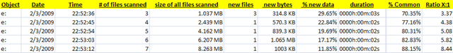
This is a long post so I decided to create a separate post for performance and replication.  To wet your appetite here are some the early numbers from the FhGFS NAS testing.

Created the above output quickly, In my follow-up performance post I will document the test bed, publish all the test variants and platform comparisons.  Stay tuned…