Garage Door Automation w/ Rev 1 Analytics

My inspiration

My family and I use our garage as the primary method of ingress and egress from our home.  Almost daily I open the garage door using the standard wall mount garage door button, I also drive away and 30 seconds later I think to myself “did I close the garage door”.  The thought of “did I close the garage door” results in one of two outcomes.

  1. I am close enough that I can strain my neck and look back over my left shoulder to see if I closed the door.
  2. I went in a direction that does not allow me to look back over my left shoulder to see the state of the door or I am too far to see the state of the door, this results in me turning around and heading home to appease my curiosity.

My Goal(s)

Initial goal:  To implement a device that allowed me to remotely check the state of my garage door and change the state of the door remotely (over the internet).  Pretty simple.

Implemented analytics add-on:  Given the intelligence of the device I was building and deploying to gather door state and facilitate state changes (open | closed) I thought wouldn’t it be cool if I captured this data and did some analytics.  E.g. – When is the door opened and closed, how long is it kept in this state and started to infer some behavioral patters.  I implemented Rev 1 of this which I will talk about below.

Planned add-ons:

  • Camera with motion capture and real-time streaming.
    Note:  Parts for this project on order and I will detail my implementation as an update to this post once I have it completed.
  • Amazon Alexa (Echo) (http://goo.gl/P3uNY6) voice control.
  • 3D printed mounting bracket (bottom of priority list)

My First Approach
Note:  This only addressed my initial design goal above.  Another reason I am glad I bagged the off-the-shelf approach and went with the maker approach.

I have automated most of my home with an ISY99i (https://goo.gl/YOklKH) and my thought was I could easily leverage the INSTEON 74551 Garage Door Control and Status Kit (http://goo.gl/Soo31V).  To make a long story short this device is a PoS so it became an AMZN return.  After doing more research on what was available off-the-shelf and aligning it with my goals I decided that I should build rather than buy.

The Build

Parts list:
Note:  Many of these parts can be changed out for similar versions.
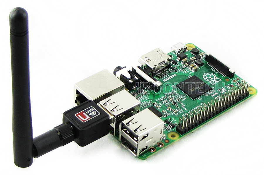
Various tools required / used:

  • Wire cutter / stripper
  • Various screwdrivers
    • Whatever you need to make connections on you garage door opener.
    • Tiny slotted screwdriver (required to tighten terminals on relay board).
  • Soldering iron
  • Heat gun (required for heat shrink)
    • Substitute a good hair dryer or lighter (be careful with lighter not to melt wires).

Planned camera add-on:
Note:  Parts ordered but have not yet arrived and this is not yet implemented.

  • 1 x Arducam 5 Megapixels 1080p Sensor OV5647 Mini Camera Video Module for Raspberry Pi Model A/B/B+ and Raspberry Pi 2 (http://goo.gl/XhCy5L)
  • 1 x White ScorPi B+, Camera Mount for your Raspberry Pi Model B+ and white Camlot, Camera leather cover (http://goo.gl/nRHvED)
    Note:  Nice to have, certainly not required.

Although below you will see my breadboard design I actually soldered and protected all final connections with heat shrink (you will see this in my post installation photos below).

Required Software
Note:  This is not a Raspberry Pi tutorial so I am going to try to keep the installation and configuration of Raspbian and other software dependencies limited to the essentials but with enough details and reference material to make getting up and running possible.

Gather requisite software and preparing to boot:

  • Download Respbian Jessie OS (https://goo.gl/BYkhLp)
  • Download Win32 Disk Imager (http://goo.gl/hz9BD)
    Note:  This is how you will write the Raspbian Image to your 8 GB microSDHC Class 4 Flash Memory Card.
    Note:  If you are not using Windows then Win32 Disk Imager is not an option.

  • Unzip the Raspbian Jessie Image and Write Image (,img file) to 8 GB microSDHC Class 4 Flash Memory Card.image
  • Insert 8 GB microSDHC Class 4 Flash Memory Card into computer open Win32 Disk Imager and write Raspbian image to microSD card (in this case drive G:)image
  • Once complete eject the microSD card from your computer and insert it into your Raspberry Pi.
  • At this time also insert your USB wireless dongle.

We are now ready to boot our Raspberry Pi for the first time bur prior to doing so we need to determine how we will connect to the console.  There are two options here.

  1. Using a HDMI connected monitor with a USB wired or wireless keyboard.
  2. Using a Serial Console (http://elinux.org/RPi_Serial_Connection)

Pick your preferred console access method from the above two options and connect and then power on the the Raspberry Pi by providing power to the the micro USB port.

Booting the raspberry Pi for the first time:

  • Default Username / Password:  pi / raspberry
  • Once the system is booted login via the console using the default Username and Password above.
  • Perform the first time configuration by executing “sudo raspi-config”
    image

    • At this point you are going to run options 1,2,3 and 9 then reboot.
    • Option 1 and 2 are self explanatory.
      • Option 1 expands the root file system to make use of your entire SD card.
      • Option 2 allows you to change the default password for the “pi” user
    • Using option 3 we will tell the Raspberry Pi to boot to the console (init level 3).
      image

      • Select option B1 and then OK.
  • Next select option 9, then A4 and enable SSH.
    image
  • Select Finish and Reboot

Once the system reboots it is time to configure the wireless networking.
Note:  I will used nano for editing, little easier for those not familiar with vi but vi can also be used.

  • Once the system is booted login via the console using the “pi” user and whatever you set the password to.
  • Enter:  “sudo –s” (this will elevate us to root so we don’t have to preface every command with “sudo”)
    image
  • To setup wireless networking we will need to edit the following files:
    • /etc/wpa_supplicant/wpa_supplicant.conf
    • /etc/network/interfaces
    • /etc/hostname
  • nano /etc/wpa_supplicant/wpa_supplicant.conf
    image
    You will likely have to add the following section:network={
    ssid=”YOURSSID”
    psk=”YOURWIRELESSKEY”
    id_str=”wireless”
    }
  • nano /etc/network/interfaces
    image
    You will likely have to edit/add the following section:
    allow-hotplug wlan0
    iface wlan0 inet manual
    wpa-roam /etc/wpa_supplicant/wpa_supplicant.confiface wireless inet static
    address [YOURIPADDRESS]
    netmask [YOUSUBNET]
    gateway [YOURDEFAULTGW]
  • nano /etc/hostname
    • Set your hostname to whatever you like, you will see I call mine “garagepi”
  • reboot
    • Once the reboot is complete the wireless networking should be working, you should be able to ping your static IP and ssh to your Raspberry Pi as user “pi”.

Raspberry Pi updates and software installs
Now that our Raspberry Pi is booted and on the network let start installing the required software.

  • ssh to the Rasberry Pi using your static IP or DNS resolvable hostname.
  • Login as “pi”
  • Check that networking looks good by executing “ifconfig”
    Note:  It’s going to look good otherwise you would not have been able to ssh to the host but if you need to check from console issuing a “ifconfig” would be a good starting place.  If you are having issues consult Google on Raspberry Pi wireless networking.
    image
  • Update Raspbian
    • sudo apt-get update
    • sudo apt-get upgrade
  • Additional software installs
    • sudo apt-get –y install git
    • sudo gem install gist
    • sudo apt-get –y install python-dev
    • sudo apt-get –y install python-rpi.gpio
    • sudo apt-get –y install curl
    • sudo apt-get –y install dos2unix
    • sudo apt-get –y install daemon
    • sudo apt-get –y install htop
    • sudo apt-get –y install vim
  • Install WebIOPi (http://webiopi.trouch.com/)
    • wget http://sourceforge.net/projects/webiopi/files/WebIOPi-0.7.1.tar.gz/download
    • tar zxvf WebIOPi-0.7.1.tar.gz
    • cd WebIOPi-0.7.1
      image
      Note:  You may need to chmod –R 755 ./WebIOPi-0.7.1
    • sudo ./setup.sh
      • Follow prompts
        Note:  Setting up a Weaved account not required.  I suggest doing it just to play with Weaved (https://www.weaved.com/) but I just use dynamic DNS and port forwarding for remote access to the device.  I will explain this more later in the post.
    • sudo update-rc.d webiopi defaults
    • sudo reboot

Once the system reports WebIOPi should be successfully installed and running.  To test WebIOPi open your browser and open the following URL:  http://YOURIPADDRESS:8000

  • You should get a HTTP login prompt.
  • Login with the default username / password:  webiopi / raspberry
  • If everything is working you should see the following:
    image

We now have all the software installed that will enable us to get status and control our garage door.  We are not going to prep for the system for the analytics aspect of the project.

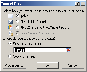
  • Create an Initial State account.
  • Once your account is created, login in and navigate to “my account” by clicking your account name in the upper right hand corner of the screen and selecting “my account”
  • Scroll to the bottom of the page and make note of or create a “Streaming Access Key”
  • As “pi” user from Raspberry Pi ssh session run the following command:  \curl -sSL https://get.initialstate.com/python -o – | sudo bash
    Note:  Be sure to include the leading “\”

    • Follow the prompts – if you say “Y” to the “Create an example script?” prompt, then you can designate where you’d like the script and what you’d like to name it.  Your Initial State username and password will also be requested so that it can autofill your Access Key.  If you say “n” then a script won’t be created, but the streamer will be ready for use.

OK all of of software prerequisites are done, let’s get our hardware built!

Shutdown and unplug the Raspberry Pi

The Hardware Build
Note:  I used fritzing (http://fritzing.org/home/) to prototype my wiring and design.  This is not required but as you can see below it does a nice job with documenting your project and also allowing you to visualize circuits prior to doing the physical soldering.  I did not physically breadboard the design, I used fritzing instead.

Breadboard Prototype

Garage_Door_bb

Connections are as follow:

  • Pin 2 (5v) to VCC on 2 Channel 5v Relay
  • Pin 6 (ground) to GND on 2 Channel 5v Relay
  • Pin 26 (GPIO 7) tom IN1 on 2 Channel 5v Relay
  • Pin 1 (3.3v) to 10k Ohm resistor to Common on Magnetic Contact Switch / Door Sensor
  • Pin 12 (GPIO 18) to 10k Ohm resistor to Common on Magnetic Contact Switch / Door Sensor
    Note:  Make sure you include the 10k Ohm resistors otherwise there will be a floating GPIO status.
  • Pin 14 (ground) to Normally Open on Magnetic Contact Switch / Door Sensor

Schematic

Garage_Door_schem

Before mounting the device and connecting the device to our garage door (our final step) let’s do some preliminary testing.

  • Power on the Raspberry Pi
  • ssh to the Rasberry Pi using your static IP or DNS resolvable hostname.
  • Lognin as “pi”
  • Open your browser and open the following URL:  http://YOURIPADDRESS:8000
    image
  • Click on “GPIO Header”
  • Click on the “IN” button next to Pin 26 (GPIO 7) (big red box around it below)
    image
  • You should hear the relay click and the LED on the relay should illuminate.
    • If this works you are in GREAT shape, if not you need to troubleshoot before proceeding.

Connect the relay to proper terminal on your garage door opener.
Note:  Garage door openers can be a little different so my connection may not exactly match your connections.  The relay is just closing the circuit just like your traditional garage door opener button.

As I mentioned above I soldered all my connections and protected them with heat shrink but there are lots of other ways to accomplish this which I talked about earlier.

Finished Product (post installation photos)Image

Above you can see the wires coming from the relay (gold colored speaker wire on the right, good gauge for this application and what I had laying around)

Below you can see the connections to the two leftmost terminals on the garage door opener (I’m a fan of sta-kons to keep things neat)

Image

Image

OK, now that our hardware device is ready to go and connected to our garage door opener let’s power it up.

Once the system is powered up let’s login as pi and download the source code to make everything work.

  • ssh to your Raspberry Pi
  • login as “pi”
  • wget https://gist.github.com/rbocchinfuso/89d406b4f83e44b2a92c/archive/cb1ccf7cb73e36502a6c3e9b4df1e1f07a70e2c6.zip
  • unzip cb1ccf7cb73e36502a6c3e9b4df1e1f07a70e2c6.zip
  • cd 89d406b4f83e44b2a92c-cb1ccf7cb73e36502a6c3e9b4df1e1f07a70e2c6
    image

Next we need to put the files in their appropriate locations.  There are no rules here but you may need to modify the source a bit if you make changes to the locations.

  • mkdir /usr/share/webiopi/htdocs/garage
  • cp ./garage.html /usr/share/webiopi/htdocs/garage
    Note:  garage.hrtml can also be places in /usr/share/webiopi/htdocs and you will not need to include /garage/ in the URL.  I use directories because I am serving multiple apps for this Raspberry Pi.
  • mkdir ~pi/daemon
  • cp garagedoor_analytics.py ~/pi/daemon
    Note:  You will need to edit this file to enter your Initial State Access Key which we made note of earlier.
  • cp garagedoor_analytics.sh ~/pi/daemon
  • cp garagedoor_analytics_keepalive.sh ~/pi/daemon

Make required crontab entries:

  • sudo crontab –e
    Note:  This edits the root crontab
  • You should see a line that looks like the following:
    #@reboot /usr/bin/startweaved.sh
    This is required to use Weaved.  If you remember earlier I said I just use port forwarding so I don’t need Weaved so I commented this out in my final crontab file.
  • Here is what my root crontab entries look like:
    #@reboot /usr/bin/startweaved.sh
    @reboot /home/pi/daemon/garagedoor_analytics_keepalive.sh
    */5 * * * * /home/pi/daemon/garagedoor_analytics_keepalive.sh

*** IMPORTANT ***  Change the WebIOPi server password.

  • sudo webiopi-passwd

Reboot the Raspberry Pi (sudo reboot)

Let’s login to the Raspberry Pi and do some testing

  • Check to see if the garagedoor_analytics.py script is running
    • ps -ef | grep garage
      image
      Looks good!
  • Open the following URL on desktop (or mobile):  http://YOURIPADDRESS/garage/garage.html
  • Login with the WebIOPi username and password which you set above.
    image
    This is what we want to see.
  • Click “Garage Door”
    image
    Confirm you want to open the door by clicking “Yes”
  • Garage door should open and status should change to “Opened”
    image
    Repeat the process to close the door.

Pretty cool and very useful.  Now for the analytics.

  • Go to the following URL: https://www.initialstate.com/app#/login
  • Login using your credentials from the account we created earlier.
  • When you login you should see something similar to the following:
    image
    Note:  “Garage Door” on the left represents the bucket where all of our raw data is being streamed to.
  • Click on “Garage Door”
    • There are number of views we can explore here.
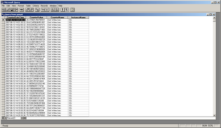
    • First lest check the raw data stream:
      image
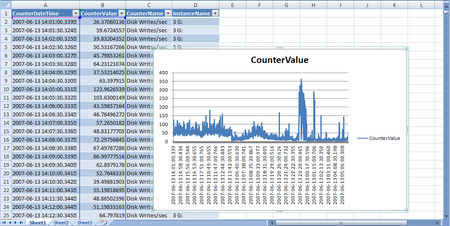
      Here we see the raw data being streamed from the Raspberry Pi to our Initial State Bucket.
    • Next lets look at some stats from the last 24 hours.
      image
      Here I can see the state of the door my time of day, the % of the day the door was opened or closed, the number of times the doo was opened, etc…

I haven’t really started mining the data yet but I am gong to place an AMP meter on the garage door and start to use this data to determine the cost associated with use of the garage door, etc…  I am thinking maybe I can do some facial recognition using the Raspberry Pi camera and OpenCV to see who is opening the door and get more precise with my analytics.

Two more item before I close out this post.

The first one being how to access the your Raspberry Pi over the internet so you can remotely check the status of your garage door and change it’s state from your mobile device.  There is really nothing special about this it’s just using dynamic DNS and port forwarding.

  • Find a good (possibly free but free usually comes with limitations and/or aggravation) dynamic DNS service.  I use a paid noip (http://www.noip.com/) account because it integrates nicely with my router, it’s reliable and I got tired of the free version expiration every 30 days.
    • This will allow you to setup a DNS name (e.g. – myhouse.ddnds.net) to reference your public IP address which assuming you have residential internet service is typically a dynamic address (meaning it can change).
  • Next setup port forwarding on your internet router to forward an External Port to an Internal IP and Port
    • This procedure will vary based on your router.
    • Remember that WebIOPi is running on port 8000 (unless you changed it) so your forwarding rule would look something like this:
      • myhouse.ddns.net:8000 >>> RPi_IP_ADDRESS:8000
      • Good article on port forwarding for reference:  http://goo.gl/apr8L

The last thing is a video walk-through of the system (as it exists today):

[youtube]https://youtu.be/Q5uizfiPBy4[/youtube]

I really enjoyed this project.  Everything from the research, building and documentation was really fun.  There were two great things for me.  The first being the ability to engage my kids in something I love, they like the hands on aspect and thought it was really cool that daddy could take a bunch of parts and make something so useful.  The second was actually having a device deployed which is extensible at a price point lower that what I have purchased an off-the-shelf solution for (understood that I didn’t calculate my personal time but the I would have paid to do the project).

My apologies if I left anything out, this was a long post an I am sure I missed something.

Looking forward to getting the camera implemented, it just arrived today so this will be a holiday project.

EMC CX3-80 FC vs EMC CX4-120 EFD

This blog is a high level overview of some extensive testing conducted on the EMC (CLARiiON) CX3-80 with 15K RPM FC (fibre channel disk) and the EMC (CLARiiON) CX4-120 with EFD (Enterprise Flash Drives) formerly know as SSD (solid state disk).

Figure 1:  CX4-120 with EFD test configuration.

image

Figure 2:  CX3-80 with 15K RPM FC rest configuration.

image

Figure 3:  IOPs Comparison

image

Figure 4:  Response Time

image

Figure 5:  IOPs Per Drive

image

Notice that the CX3-80 15K FC drives are servicing ~ 250 IOPs per drive, this exceeds 180 IOPs per drive (the theoretical maximum for a 15K FC drive is 180 IOPs) this is due to write caching.  Note that cache is disabled for the CX4-120 EFD tests, this is important because high write I/O load can cause something known as a force cache flushes which can dramatically impact the overall performance of the array.  Because cache is disabled on EFD LUNs forced cache flushes are not a concern.

Table below provides a summary of the test configuration and findings:

Array CX3-80 CX4-120
Configuration (24) 15K FC Drives (7) EFD Drives
Cache Enabled Disabled
Footprint   ~42% drive footprint reduction
Sustained Random Read Performance   ~12x increase over 15K FC
Sustained Random Write Performance   ~5x increase over 15K FC

In summary, EFD is a game changing technology.  There is no doubt that for small block random read and write workloads (i.e. – Exchange, MS SQL, Oracle, etc…) EFD dramatically improves performance and reduces the risk of performance issues.

This post is intended to be an overview of the exhaustive testing that was performed.  I have results with a wide range of transfer sizes beyond the 2k and 4k results shown in this posts, I also have Jetstress results.  If you are interested in data that you don’t see in this post please Email me a rbocchinfuso@gmail.com.

Benchmarking De-Duplication and with Databases

In the interest of benchmarking de-duplication rates with databases I created a process to build a test database, load test records, dump the database and perform a de-dupe backup using EMC Avamar on the dump files.  The process I used is depicted in the flowchart below.

image

1.  Create a DB named testDB
2.  Create 5 DB dump target files – testDB_backup(1-5)
3.  Run the test which inserts 1000 random rows consisting of 5 random fields for each row.  Once the first insert is completed a dump is performed to testDB_backup1.  Once the dump is complete a de-dupe backup process is performed on the dump file.  This process is repeated 4 more times each time adding an additional 1000 rows to the database and dumping to a new testDB_backup (NOTE:  this dump includes existing DB records and the newly inserted rows) file and performing the de-dupe backup process.

Once the backup is completed a statistics file is generated showing the de-duplication (or commonality) ratios.  The output from this test is as follows:

image

You can see that each iteration of the backup shows an increase in the data set size with increasing commonality and de-dupe rations.  This test shows that with 100% random database data using a DB dump and de-dupe backup strategy can be a good solution for DB backup and archiving.

OS X as Vista VMware Guest OS

I am now successfully running OS X as a VMware Guest OS. This was just a Sunday afternoon project to kill some free time… The UI is a bit slow and the networking requires a little tweaking to get it working but other than that everything works OK out of the box. To get more information on how to do this check out this link.

Here a screen shot of my Vista desktop running OS X:

image

Windows and mount points…

Those of us who used CP/M and DOS in the early days became accustomed to drive letters which BTW was a good design when most systems has two maybe three devices. The same computer enthusiasts who used CP/M and DOS most likely through education or professional experience were introduced to UNIX at some point. If you are like me this was probably during your college years, we began to realize how much more elegant the UNIX operating system was with novel ideas such as “mount points”, well Microsoft sorta figured this out a few years ago and integrated mount points into Windows. To me there is absolutely no reason that anyone in the server space should be using drive letters (Excluding A:,B:,C: and D: of course) unless legacy applications are hard coded to use drive letters and the move to mount points is just too painful (unfortunately in the past drive letters were the only way to address storage devices, if you are still doing this for new applications shame, shame!). One issue with mount points is an inability to easily determine total, used, and free space for a physical device from Windows Explorer. While I use mount points almost exclusively, many of my customers complain of the need to drop to the CLI (only a complaint you would hear in the Windows world…. although I agree it is nice to have a single view of all physical devices, like that provided by Windows Explorer). They could open Disk Management but that too is kind of cumbersome to just view available space. Here is a small VB script that I wrote that will provide total, used and free space for physical devices by enumerating the devices that match a specific drive label:

——— SCRIPT STARTS HERE ———

WScript.Echo “B2D Capactiy Reporter – ” & Date
Wscript.Echo “RJB – 1/2/2008”
Wscript.Echo “———————————–”

Dim totalB2D, totalUSED, totalFREE
totalB2D = 0
totalUSED = 0
totalFREE = 0

strComputer = “.”
Set objWMIService = GetObject(“winmgmts:” _
& “{impersonationLevel=impersonate}!\\” & strComputer & “\root\cimv2”)

Set colItems = objWMIService.ExecQuery(“Select * from Win32_Volume where label like ‘b2d%‘”)

For Each objItem In colItems
WScript.Echo “Label: ” & objItem.Label
WScript.Echo “Mount Point: ” & objItem.Name
WScript.Echo “Block Size: ” & (objItem.BlockSize / 1024) & “K”
WScript.Echo “File System: ” & objItem.FileSystem
WScript.Echo “Capacity: ” & round(objItem.Capacity / 1048576 / 1024,2) & ” GB”
WScript.Echo “Used Space: ” & round((objItem.Capacity – objItem.FreeSpace) / 1048576 / 1024,2) & ” GB”
WScript.Echo “Free Space: ” & round(objItem.FreeSpace / 1048576 / 1024,2) & ” GB”
WScript.Echo “Percent Free: ” & round(objItem.FreeSpace / objItem.Capacity,2) * 100 & ” %”
totalB2D = totalB2D + (objItem.Capacity / 1048576 / 1024)
totalFREE = totalFREE + (objItem.FreeSpace / 1048576 / 1024)
totalUSED = totalUSED + ((objItem.Capacity – objItem.FreeSpace)/ 1048576 / 1024)
Wscript.Echo “———————————–”
Next

WScript.Echo “———————————–”
WScript.Echo “Total B2D Capacity: ” & round(totalB2D / 1024,2) & ” TB”
WScript.Echo “Total Used Capacity: ” & round(totalUSED / 1024,2) & ” TB”
WScript.Echo “Total Free Capacity: ” & round(totalFREE / 1024,2) & ” TB”
WScript.Echo “Total Percent Free: ” & round(totalFREE / totalB2D,2) * 100 & ” %”

——— SCRIPT ENDS HERE ———

This script was originally written to report the utilization of devices that were being used as Backup-to-Disk targets, hence the name B2D Capacity Reporter. The scripts keys on the disk label so it is important to label the disks properly so that it will report accurately (this can be done from Disk Management or the Command line). I have bolded above the only change that really needs to be made to make the script function properly. This script could easily be modified to report across multiple systems which could be useful if you are looking to tally all the space across multiple servers.

I have only tested this on Windows 2003 so I am not sure how it will function on other versions of Windows. Enjoy!

Oh, one more thing. When you save the script be sure to run it with cscript not wscript (e.g. – cscript diskspace.vbs).

The Cache Effect

Following a fit of rage last night after I inadvertently deleted 2 hours worth of content I have now calmed down enough to recreate the post.

The story starts out like this, a customer who recently installed a EMC CX3–80 was working on a backup project roll out, the plan was to leverage ATA capacity in the CX3–80 as a backup-to-disk (B2D) target.  Once they rolled out the backup application they were experiencing very poor performance for the backup jobs that were running to disk, additionally the customer did some file system copies to this particular device and the performance appeared to slow.

The CX3–80 is actually a fairly large array but for the purposes of this post I will focus on the particular ATA RAID group which was the target of the backup job where the performance problem was identified.

I was aware that the customer only had on power rail due to some power constraints in their current data center.  The plan was to power up the CX using just the A side power until they could de-commission some equipment and power on the B side.  My initial though was that cache the culprit but I wanted to investigate further before drawing a conclusion.

My first step was to log into the system and validate that cache was actually disabled, which it was.  This was due to the fact that the SPS (supplemental power supply) only had one power feed and the batteries where not charging.  In this case write–back cache is disabled to protect from potential data loss.  Once I validated that cache was in fact disabled I thought that I would take a scientific approach to resolving the issue by base lining the performance without cache and then enabling cache and running the performance test again.

The ATA RAID group which I was testing on was configured as a 15 drive R5 group with 5 LUNs (50 – 54) ~ 2 TB in size.

Figure 1:  Physical disk layout

R5

My testing was run against drive f: which is LUN 50 which resides on the 15 drive R5 group depicted above.  LUNs 51, 52, 53 and 54 were not being used so the RG was only being used by the benchmark I was running on LUN 50.

Figure 2:  Benchmark results before cache was enabled

Pre-cache

As you can see the performance for writes is abysmal.  I will focus on the 64k test as we progress through the rest of this blog.  You will see above that the 64k test only push ~ 4.6 MB/s.  Very poor performance for a 15 drive stripe.  I have a theory for why this is but I will get to that later in the post.

Before cache couple be enabled we needed to power the second power supply on the the SPS, this was done by plugging the B power supply on the SPS into the A side power rail.  Once this was complete and the SPS battery was charged cache was enabled on the CX and the benchmark was run a second time.

Figure 3:  Benchmark results post cache being enabled (Note the scale on this chart differs from the above chart)

Post-cache

As you can see the performance increased from ~ 4.6 MB/s for 64k writes to ~ 160.9 MB/s for 64k writes.  I have to admit I would not have expected write cache to have this dramatic of an effect.

After thinking about it for a while I formulated some theories that I hope to fully prove out in the near future.  I believe that the performance characteristics that presented themselves in this particular situation was a combination of a number of things, the fact that the stripe width was 15 drives and cache being disabled created the huge gap in performance.

Let me explain some RAID basics so hopefully the explanation will become a bit clearer.

A RAID group had two key components that we need to be concerned with for the purpose of this discussion:

  1. Stripe width – which is typically synonymous with the number of drives in the the raid group
  2. Stripe depth – which is the size of the write that the controller performs before it round robin to the next physical spindle (Depicted in Figure 4)

Figure 4: Stripe Depth

Stripe_depth

The next concept is write cache, specifically two features of write cache know as write-back cache and write-gathering cache.

First lets examine the I/O pattern without the use of cache.  Figure 5 depicts a typical 16k I/O on an array with and 8k stripe depth and a 4 drive stripe width, with no write cache.

Figure 5:  Array with no write cache

No_cache

The effect of no write cache is two fold.  First there is no write-back so the I/O needs to be acknowledge by the physical disk, this is obviously much slower that and ack from memory.  Second, because there is no write-gathering full-stripe writes can not be facilitated which means more back-end I/O operations, affectionately referred to as the Read-Modify-Write penalty.

Now lets examine the same configuration with write-cache enabled.  Depicted in Figure 6.

Figure 6:  Array with write cache enabled

W_cache

Here you will note that acks are sent back to the host before they are written to physical spindles, this dramatically improves performance.  Second write-gathering cache is used to facilitate full-stripe writes which negates the read-modify-write penalty.

Finally my conclusion is that the loss of write cache could be somewhat negated by reducing stripe widths from 15 drives to 3 or 4 drives and creating a meta to accommodate larger LUN sizes.  With a 15 drive raid group the read-modify-write penalty can be severe as I believe we have seen in Figure 2.  This theory needs to be test, which I hope to do in the near future.  Obviously write-back cache also had an impact but I am not sure that is was as important as write-gathering in this case.  I could have probably tuned the stripe-depth and file system I/O size to improve the efficiency without cache as well.

Performance Analysis

So let me set the stage for this blog. I recently completed a storage assessment for a customer. Without boring you with the details one of the major areas of concern was the Exchange environment, I was provided with proem data from two active Exchange cluster member to be used for analysis. The proem data was collected on both cluster members over the course of a week at 30 second intervals – THAT’S ALOT OF DATA POINTS. Luckily the output was provided in .blg (binary log) format because I am not sure how well Excel would have handled opening a .CSV file with 2,755,284 rows – YES you read that correctly 2.7 million data points – and that was after I filtered the counters that I did not want.

The purpose of this post is to walk through how the data was ingested and mined to produce useful information. Ironically having such granular data point while annoying at the onset proved to be quite useful when modeling the performance.

First let’s dispense with some of the requirements:

  • Windows XP, 2003
  • Windows 2003 Resource Kit (required for the log.exe utility)
  • MSDE, MSSQL 2000 (I am sure you can use 2005 – but why – it is extreme overkill for what we are doing)
  • A little bit of skill using osql
    • If you are weak 🙂 and using MSSQL 2000 Enterprise Manager can be used
  • A good SQL query tool
  • MS Excel (I am using 2007 – so the process and screen shots may not match exactly if you are using 2003, 2000, etc…)
    • Alternatively a SQL reporting tool like Crystal could be used. I choose Excel because the dataset can easily be manipulated once in a spreadsheet.
  • grew for Windows (http://gnuwin32.sourceforge.net/packages/grew.htm) – ensure this is in your path

OK – now that the requirements are out of the way let’s move on. I am going to make the assumption that the above software is installed and operational, otherwise this blog will get very, very long. NOTE: It is really important that you know the “sa” password for SQL server.

Beginning the process:

Step 1: Create a new data base (my example below uses the data base name “test” – you should use something a bit more descriptive)

Microsoft Windows XP [Version 5.1.2600]
(C) Copyright 1985-2001 Microsoft Corp.

C:\Documents and Settings\bocchrj>osql -Usa
Password:
1> create database test
2> go
The CREATE DATABASE process is allocating 0.63 MB on disk ‘test’.
The CREATE DATABASE process is allocating 0.49 MB on disk ‘test_log’.
1> quit

C:\Documents and Settings\bocchrj>

NOTE: This DATABASE will be created in the default DATA location under the SQL SVR install directory. Make sure you have enough capacity – for my data set of 2.7 million rows the database (.mdf) was about 260 MB.

Step 2: Create an ODBC connection to the database

A nice tutorial on how to do this can be found here: http://www.truthsolutions.com/sql/odbc/creating_a_new_odbc_dsn.htm

Two things to note:

  • Use the USER DSN
  • Use SQL Server Authentication (NOT NT Authentication) the user name is “sa” and hopefully you remembered the password.

Step 3: Determine relevant counters

Run the following command on the .blg file: log -q perf.blg > out.txt

This will list all of the counters to the text file out.txt. Next open counters.txt in you favorite text editor and determine which counters are of interest (NOTE: Life is much easier if you import a specific counter class into the database, create new a new database for a new counter class)

Once you determine the counter class e.g. PhysicalDisk run: log -q perf.blg | grew PhysicalDisk > counters.txt

Step 3: Import the .blg into the newly created database.

  • NOTE: There are two considerations here

    • Are the data points contained in a single .blg file (if you have 2.7 million data points this is unlikely)? If they are the command to do the import is fairly simple:

      • log perf.blg -cf counter.txt -o SQL:DSNNAME!description

    • If the data points are contained in a number of files make sure that these files are housed in the a directory. You can use the following PERL script to automate the import process (NOTE: This requires that PERL be installed – http://www.activestate.com/Products/ActivePerl/)

#!/usr/bin/perl -w

# syntax: perl import_blg.pl input_dir odbc_connection_name $counter
# e.g. – perl import_blg_pl

#DO NOT EDIT BELOW THIS LINE
$dirtoget=”$ARGV[0]”;
$odbc=”$ARGV[1]”;
$counter=”$ARGV[2]”;
$l=0;

opendir(IMD, $dirtoget) || die(“Cannot open directory”);
@thefiles= readdir(IMD);
closedir(IMD);

foreach $f (@thefiles)
{
unless ( ($f eq “.”) || ($f eq “..”) )
{
$label=$l++;
system “log \”$dirtoget\/$f\” -cf $counter -o SQL:$odbc!$label”;
}
}


  • If the import is working properly you should see output similar to the following:

Input
—————-
File(s):
C:\perf_log – 30 second interval_06132201.blg (Binary)

Begin: 6/13/2007 22:01:00
End: 6/14/2007 1:59:30
Samples: 478

Output
—————-
File: SQL:DSNNAME!1.blg

Begin: 6/13/2007 22:01:00
End: 6/14/2007 1:59:30
Samples: 478

The command completed successfully.

Step 4: OK – The data should now be imported into the database. We will now look at the DB structure (table names) and run a test query. At this point I typically start using SQL Manager 2005 Lite but you can continue to use osql or Enterprise Manager (uggghhhh). For the purposes of cutting and pasting examples I used osql.

  • This is not a DB 101 tutorial but you will need to be connected to the database we created earlier.

  • Once connected run the following query (I cut out non relevant information in the interest of length):

C:\Documents and Settings\bocchrj>osql -Usa
Password:
1> use test
2> go
1> select * from subjects where type = ‘u’ order by name
2> go
CounterData
CounterDetails
DisplayToID

(3 rows affected)
1>

CounterData and CounterDetails are the two tables we are interested in:

Next lets run the query to display the first 100 rows of the CounterDetails table to verify that the data made its way from the .blg file to the database

1> select top 20 * from counterdetails
2> go
SHOULD SCROLL 20 RECORDS
(20 rows affected)
1>quit

Step 5: Determining what to query

Open counters.txt in your favorite browser and determine what you want to graph – there are a number of metrics, pick one you can get more complicated once you get the hang of the process.

e.g. When you open the text file you will see a number of rows that look like this – Take note of bold sections below, this is the one of the filters that will be used when selecting the working dataset

\test\PhysicalDisk(4)\Avg. Disk Bytes/Read
\test\PhysicalDisk(5)\Avg. Disk Bytes/Read
\test\PhysicalDisk(6 J:)\Avg. Disk Bytes/Read
\test\PhysicalDisk(1)\Avg. Disk Bytes/Read
\test\PhysicalDisk(_Total)\Avg. Disk Bytes/Read
\test\PhysicalDisk(0 C:)\Avg. Disk Write Queue Length
\test\PhysicalDisk(3 G:)\Avg. Disk Write Queue Length
\test\PhysicalDisk(4)\Avg. Disk Write Queue Length
etc…

Once you determine which performance counter is of interest open Excel.

Step 6: Understanding the anatomy of the SQL query

SELECT
CounterData.”CounterDateTime”, CounterData.”CounterValue”,
CounterDetails.”CounterName”, CounterDetails.”InstanceName”
FROM
{ oj “test“.”dbo”.”CounterData” CounterData INNER JOIN “test“.”dbo”.”CounterDetails” CounterDetails ON
CounterData.”CounterID” = CounterDetails.”CounterID”}
WHERE
CounterDetails.”InstanceName” = ‘3 G:‘ AND CounterDetails.”CounterName”=’Disk Writes/sec‘ AND CounterData.”CounterDateTime” like ‘%2007-06-13%’

  • The above query will return all the Disk Writes/sec on 6/13/2007 for the G: drive.
  • In the above query I have BOLDED the VARIABLES that should be modified when querying the database. The JOINS should NOT be modified. You may add additional criteria like multiple INSTANCENAME or COUNTERNAME fields to grab, etc…. Below you will see exactly how to apply the query.

Step 7: Run the query from Excel (NOTE: Screen shots are of Excel 2003, the look and feel will be different for other versions of Excel)

ex-query1

Once you select “From Microsoft Query” the next screen will appear

dsn

Select the DSN that you defined earlier. NOTE: Also uncheck the “Use the Query Wizard to create/edit queries. I will provide the query syntax which will make life much easier.Now you need to login to the database. Hopefully you remember the sa password.

login add

Once the login is successful – CLOSE the add tables window

Now you will see the MS Query Tool Click the SQL button on the toolbar. Enter the SQL query into the SQL text box and hit OK. You will recite a warning – just hit OK and continue.

Use the query syntax explained above.

sql

Once the query is complete it will return a screen that looks like this:

q

Now hit the 4th button from the left on the tool bar “Return Data” – this will place the data into Excel so that is can be manipulated:

e

Once the data is placed into Excel you can begin to graph and manipulate it.

out

I hope this was informative, if you find any errors in the process please place a comment to the post.

vmfs and rdm performance characteristics

It seems as if one of the most debated topics related to VMware and I/O performance is the mystery sounding the relative performance characteristics of vmfs volumes and rdm (Raw Device Mode) volumes.

Admittedly it is difficult to argue with the flexibility and operational benefits of vmfs volumes but I wanted to measure the characteristics of each approach and provide some documentation that could be leveraged when making the decision to use vmfs or rdm.? By no means are these test concluded but I thought as a gathered the data I would blog it so it could be used prior to me completing the whitepaper which all these tests will be part of.

Benchmark configuration:
The benchmarks contained in this document were performed in a lab environment with the following configuration:

  • Physical Server:? Dell dual CPU 2850 w/ 4 GB RAM
    • Windows 2003 SP2 Virtual Machine
    • Single 2.99 Ghz CPU
    • 256 MB RAM (RAM configured this low to remove the effects of kernel file system caching)
  • Disk array
    • EMC CLARiiON CX500
    • Dedicated RAID 1 Device
    • 2 LUNs Created on the RAID 1 Storage Group
    • Two dedicated 10 GB file systems
      • c:\benchmark\vmfs
        • 10 GB .vmdk created and vmfs and NTFS file system created
      • c:\benchmark\rdm
        • 10 GB rdm volume mapped to VM and NTFS file system created?

Benchmark tools:
Benchmark tests thus far were run using?two popular?disk and file system benchmarking tools.

IOzone Benchmarks:

HDtune benchmarks:

HD Tune: VMware Virtual disk Benchmark
Transfer Rate Minimum : 54.1 MB/sec
Transfer Rate Maximum : 543.7 MB/sec
Transfer Rate Average : 476.4 MB/sec
Access Time : 0.4 ms
Burst Rate : 83.3 MB/sec
CPU Usage : 36.9%

HD Tune: DGC RAID 1 Benchmark
Transfer Rate Minimum : 57.1 MB/sec
Transfer Rate Maximum : 65.3 MB/sec
Transfer Rate Average : 62.4 MB/sec
Access Time : 5.4 ms
Burst Rate : 83.9 MB/sec
CPU Usage : 13.8%

One thing that is very obvious is that VMFS makes extensive use of system/kernel cache.? This is most obvious in the HDtune benchmarks.? The increased CPU utilization is a bit of a concern, most likely due to the caching overhead.? I am going to test small block random writes while monitoring CPU overhead, my gut tells me that small block random writes to a VMFS volume will tax the CPU.? More to come….

Preliminary results: rsych to replicate virtual machines

So a couple of months ago or so I had the idea to test and document the use of rsych to replicate VMware virtual machines. Unfortunately my machine is running ESX 2.5.x and I had yet to upgrade to 3.0 so this information is a bit depreciated but I feel that it will be indicative of what I will see on ESX 3.0 (aka – VI3). On ESX 3.0 the process actually becomes much easier because all of the files (.vmx, .vmdk, .nvram) are contained in the same directory structure. So here is a simplistic representation of the commands required to replicate a VM on ESX 2.5, I am also in the process of building an automation script for ESX 3.0:

************ CREATE .REDO LOG ************
ware-cmd ~bocchrj/vmware/rh62_1/linux.vmx addredo scsi0:0

************ STARTING REPLICATION ************
rsync –verbose –progress –stats –compress /vmfs/VMs/rh62_1.vmdk esx2::rsyncVMs

************ REPLICATE VM CONFIG FILES ************
rsync –verbose –progress –stats –compress /home/bocchrj/vmware/rh62_1/* esx2::vmconfig/rh62_1

************ ADDING REDO.REDO LOG ************
vmware-cmd ~bocchrj/vmware/rh62_1/linux.vmx addredo scsi0:0

************ COMMITING REDO LOGS *************
vmware-cmd ~bocchrj/vmware/rh62_1/linux.vmx commit scsi0:0 1 0 1
vmware-cmd ~bocchrj/vmware/rh62_1/linux.vmx commit scsi0:0 0 0 0

************ DONE ************

The process worked well. I captured the output of the initial rsync and the second rsych cycle below:

Initial rsync cycle

Number of files: 1
Number of files transferred: 1
Total file size: 419430912 bytes
Total transferred file size: 419430912 bytes
Literal data: 419430912 bytes
Matched data: 0 bytes
File list size: 30
File list generation time: 0.152 seconds
File list transfer time: 0.000 seconds
Total bytes sent: 85826493
Total bytes received: 38

sent 85826493 bytes received 38 bytes 432375.47 bytes/sec
total size is 419430912 speedup is 4.89

Second rsync cycle

Number of files: 1
Number of files transferred: 1
Total file size: 419430912 bytes
Total transferred file size: 419430912 bytes
Literal data: 1864192 bytes
Matched data: 417566720 bytes
File list size: 30
File list generation time: 0.135 seconds
File list transfer time: 0.000 seconds
Total bytes sent: 344586
Total bytes received: 143405

sent 344586 bytes received 143405 bytes 4337.70 bytes/sec
total size is 419430912 speedup is 859.51

Looking forward to getting sometime to play with this on ESX 3.0, I am lobbying hard for the 48hr day 🙂

Mounting .vmdk files in Windows

Ever feel the need to mount a Windows or Linux .vmdk on windows, I have. Here are a couple of utilities that make it possible to open Linux and Windows .vmdks on Windows in read-only mode or read/write mode.

Virtual Disk Driver for Windows (http://chitchat.at.infoseek.co.jp/vmware/vdk.html)
Ext2IFS – Ext2/3 file system driver for windows. Required to mount Linux Virtual disks on windows (http://www.fs-driver.org/index.html)